Week 2 (5/31 - 6/6) Research Log

I started off this week by presenting an overview of my project to my peers in the REU program (the slides for this presentation can be found here).

This week I encountered some difficulties while attempting to preprocess the melt pool data that will be fed into our classification model. The VGG16 model we will be using requires that inputs be in the form of three-channel rgb images; the data I am working with is from single-channel thermal images and is stored in CSV files. From what I can tell by searching for resources online this seems to be a somewhat unique scenario, but I eventually found a package called plantcv (which was developed by scientists who use thermal imaging to classify plants). The plantcv documentation had a tutorial for the CSV-to-rgb conversion I needed. I installed the package and after resolving (many) conflicting dependencies, I tested it out on one of my CSV files to somewhat underwhelming results; the melt pool is visible in the intermediate grayscale image, but the artificially colored rgb image is just completely yellow. I intend to discuss potential resolutions to this issue with Dr. Guo during our Monday meeting next week.

This week I also set up a virtual python environment for my model to run in, installed and resolved dependency conflicts for all of the python packages I will need, and was able to successfully use a pre-trained VGG16 model to classify an image.

Week 3 (6/7 - 6/13) Research Log

This week I attended the TRIPODS Data Science Bootcamp and learned a lot about creating data visualizations, building regression models, and experiment design.

This week I also encountered a few challenges while preprocessing the data, particularly when it came to pseudocoloring the images so that they matched the examples I was trying to emulate (since most of the temperature values in each image are very close together with only a select few at 0, I ended up scaling matplotlib’s “jet” colormap so that the minimum value was 150 rather than 0 in order to create images that used the entire spectrum of the colormap). It also took some experimenting to end up with an image of a data type that could be saved in a format that a VGG16 model would be able to interpret correctly.

Eventually, I finished preprocessing the data (converting all of the CSV files to RGB images that resembled those from Dr. Guo’s paper “A physics-driven deep learning model for process-porosity causal relationship and porosity prediction with interpretability in laser metal deposition”). Subsequently, I was able to move on to applying transfer learning techniques to a pre-trained VGG16 model that comes with Keras.

Week 4 (6/14 - 6/20) Research Log

One of Dr. Guo’s papers, "A physics-driven deep learning model for process-porosity causal relationship and porosity prediction with interpretability in laser metal deposition" [10], states that for the original PyroNets, “the 1557 pyrometer images [were] randomly split into an initial training set (1237 good and 61 bad images) and a test set (247 good and 12 bad images).” While writing a Python script to randomly sort the images into training and test sets with these breakdowns, I noticed that the dataset I was working with had 2 more good images and 2 fewer bad images than the dataset outlined in the paper. To adjust for this, I randomly split the images into an initial training set containing 1237 good and 59 bad images (as the bad ones would be bootstrapped later) and a test set containing 249 good and 12 bad images. To account for the imbalance between the good and bad classes in the training set, I developed an algorithm to bootstrap (i.e. create augmented copies of the original bad images so that there would be an equal number of images in each class) the training data that belongs to the “bad” porosity class. After testing a few bootstrapping techniques (such as vertical and horizontal shifts), I settled on creating copies of the original images that were slightly rotated to ensure that no pixels would be shifted off of the image.

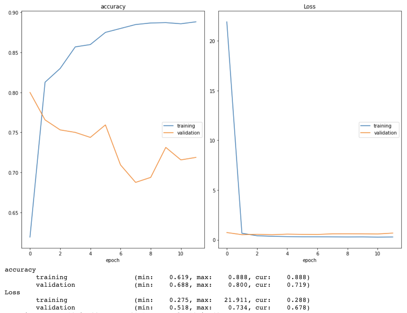
Moreover, I used a transfer learning strategy to begin training my model. After successfully connecting to a remote GPU via Google Colab, I loaded the pre-trained (on ImageNet data, not our data) VGG16 model from the Keras library into my environment and used the Keras ImageDataGenerator class and flow_from_directory method to preprocess the images and create training, validation, and test generators. Using a batch size of 64 and the Adam optimizer with a learning rate of 0.001, I began training the pre-trained model on our dataset. I used ModelCheckpoint and EarlyStopping to save the best version of the model and restore the weights with the lowest validation loss once the model began overfitting, respectively. I also implemented a real time plot of both training and validation accuracy and loss in order to gain a better understanding of how well the model was learning (see example below). It quickly became clear that the model was overfitting. I have begun researching ways to prevent this, and intend to discuss the issue with Dr. Guo at our next meeting.

Week 5 (6/21 - 6/27) Research Log

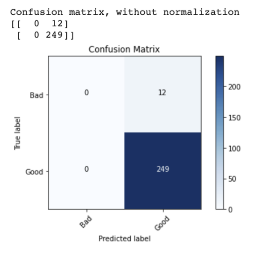
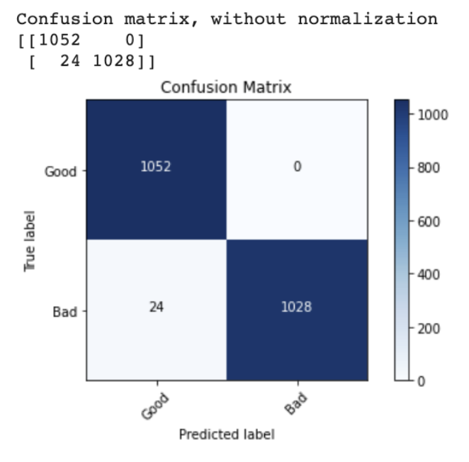
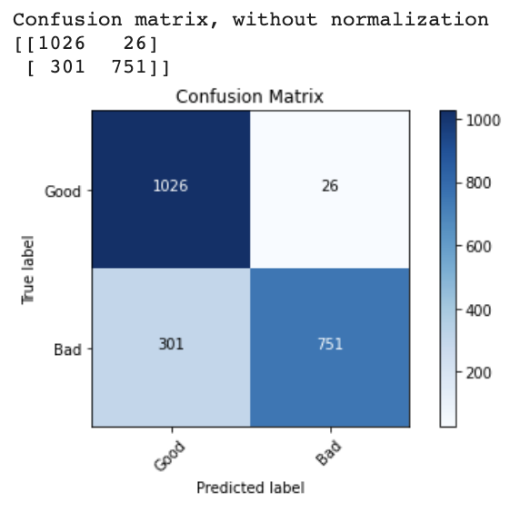
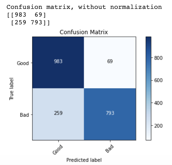
First, to gain further insight into why my transfer learning model was overfitting, I plotted confusion matrix using matplotlib and sklearn metrics and found that the model was predicting “good” for every image in the test set (and that this just happened to deceptively be 95% accurate).

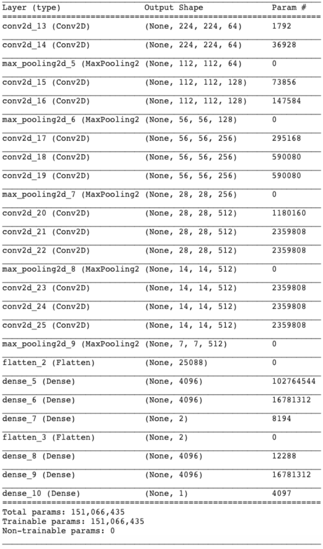
I then attempted to freeze the weights of the earlier layers in the pre-trained VGG16 model while allowing the later layers to be trainable by our new data, but this did not improve performance. From there, I decided to create a VGG16 model from scratch and train it only on our pyrometer image dataset (see model summary below).

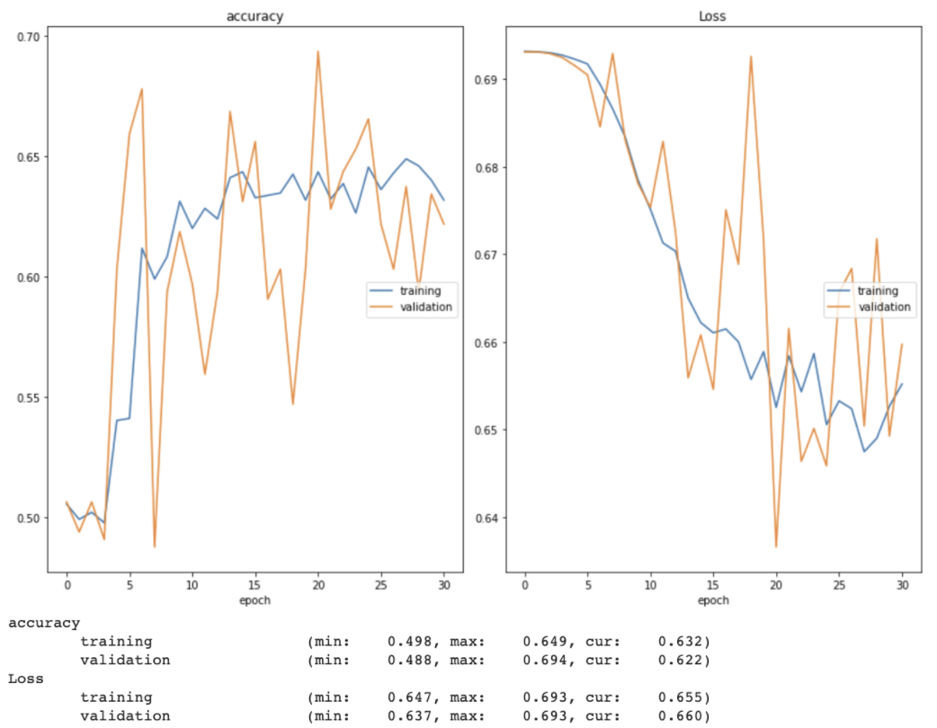
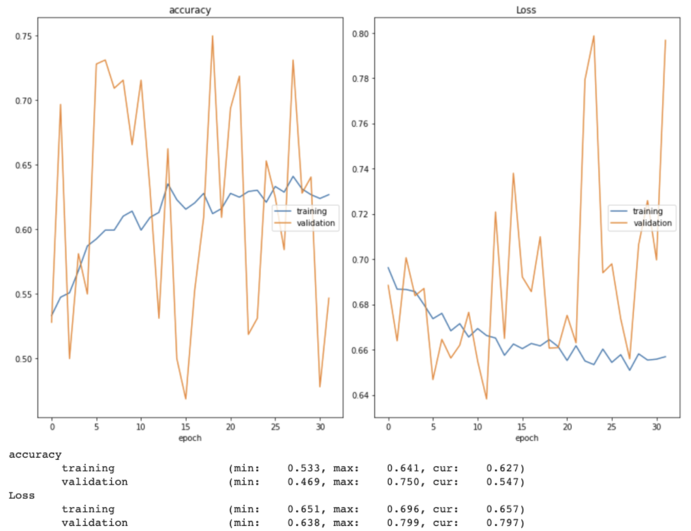
The accuracy of this model, however, plateaued at around 65%. As you can see below, the early stopping method stopped the initial training session just after 30 epochs. Even after reloading the best weights from the initial training session and continuing to train the model for 30 more epochs, both training and validation accuracy had plateaued below 70%.

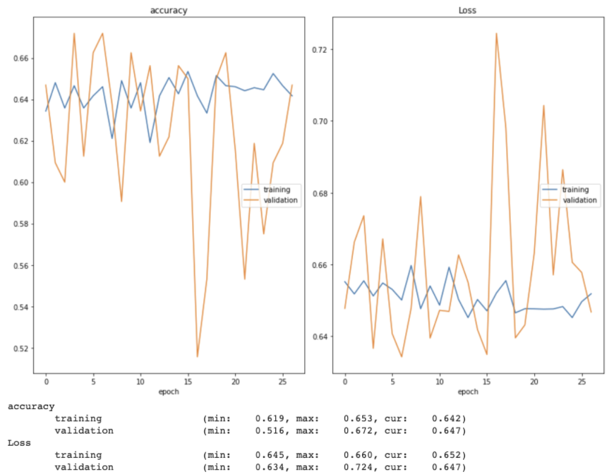
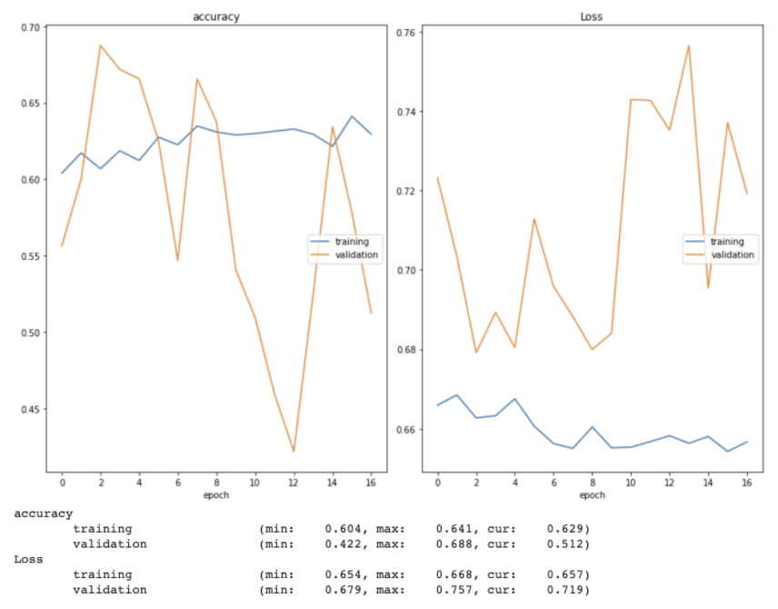
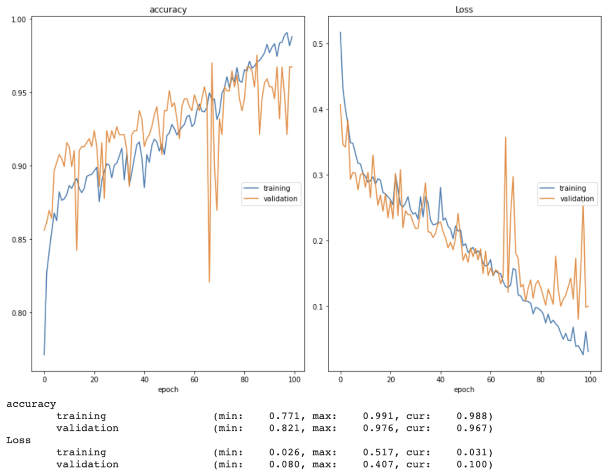
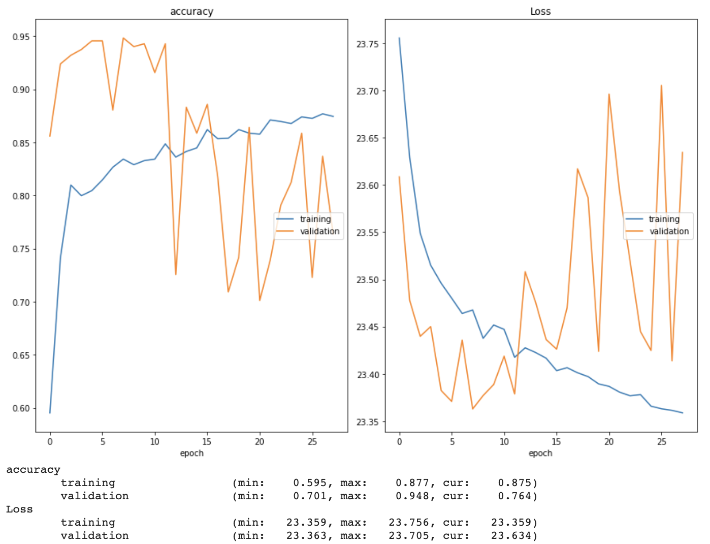
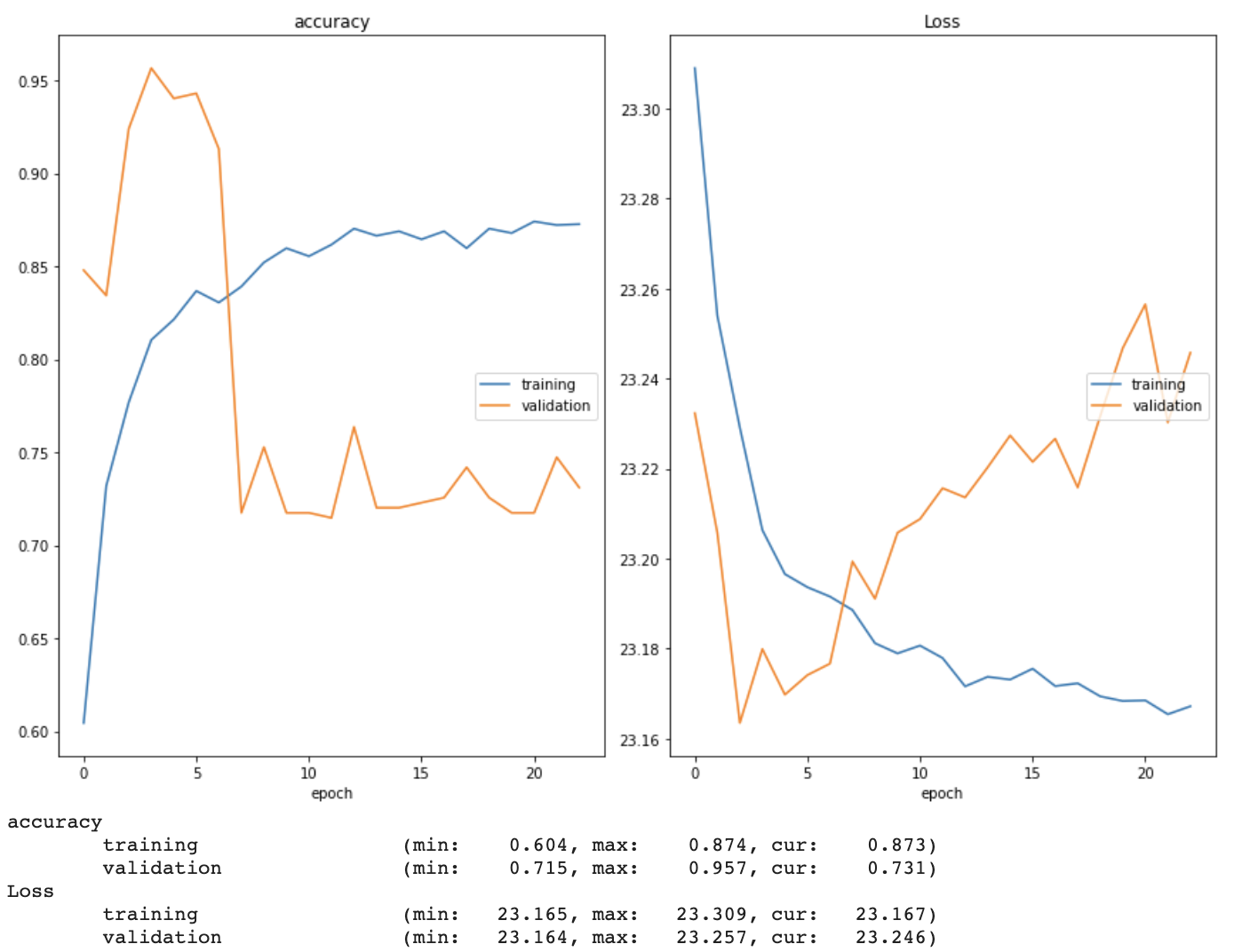
While fine tuning the model, I tried both increasing and decreasing the learning rate (and implementing a learning rate scheduler that decreased an initial learning rate of 0.001 over time). I also allowed the model to train for more epochs without early stopping, changed the loss function from categorical crossentropy to binary crossentropy (and swapped the softmax layer to a sigmoid one to match), explored one-hot encoding the image labels, switched the optimizer from Adam to SGD, and added dropout layers between the fully-connected layers. I used a real time plot of both training and validation accuracy and loss as well as confusion matrices to monitor how well the model was learning. Two examples of these training and validation accuracy and loss plots can be seen below.

Finally, I conducted a training session using simple training and validation sets that consisted of one good and one bad image each to ensure that the model was even capable of reaching 100% accuracy on any dataset, and that there was not some underlying issue with the model architecture itself. The model was indeed able to reach 100% accuracy with this dataset.

Week 6 (6/28 - 7/4) Research Log

I began this week by reading “Deep Learning-Based Data Fusion Method for In Situ Porosity Detection in Laser-Based Additive Manufacturing” [8], which gave a more detailed description of the original PyroNets. After ensuring that my model architecture matched that of those original PyroNets (including switching the binary crossentropy loss function back to categorical crossentropy), I continued to fine tune my model. I found that the most dramatic improvement in accuracy resulted from decreasing the batch size from 64 to 16. I also removed the image augmentation commands from my training set generator, as I realized that they were augmenting some images for the second time (since many of the bad images were bootstrapped).

At this point, the model still overfit fairly quickly while training, and I had a sneaking suspicion that the dataset, rather than the model architecture or settings, was the main culprit. Thus, I tried undersampling by training the model on a subset of the training set that included 59 good images and the 59 original bad images (no bootstrapped images). While the model of course was not able to achieve the same level of accuracy as it had when it trained on thousands of images, it did not overfit as severely this time. I suspect that my choice of bootstrapping method for the bad images (rotating each image by a random number of degrees) had the unintended effect of cropping out some of the relevant porous pixels. Subsequently, I bootstrapped the 59 bad images in the training set again, this time using a combination of horizontal flips, vertical flips, and brightness shifts instead of rotations.

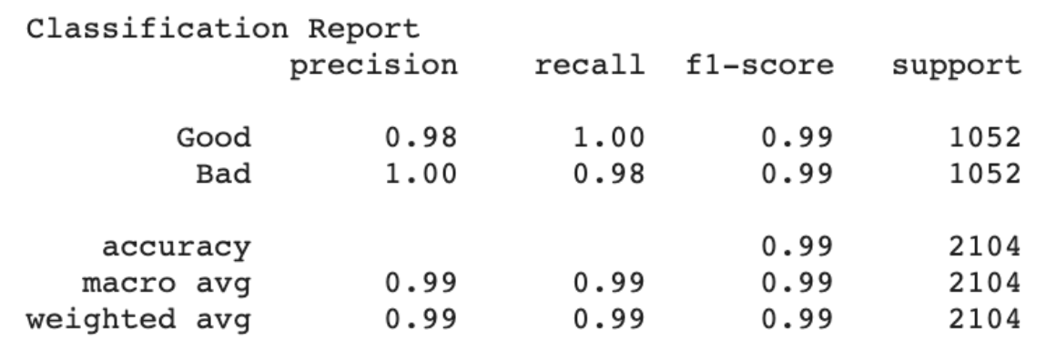
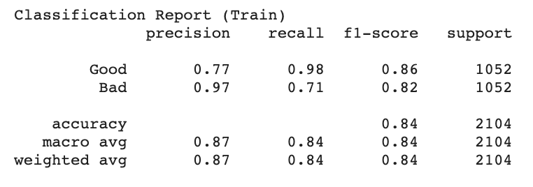
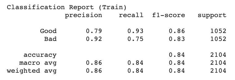
After all of these changes, my model was able to achieve 98.8% accuracy on the training set and 96.7% accuracy on the validation set. Specifically, only 24 images in the training set (all bad images) were misclassified. Since there were 59 original (non-bootstrapped) bad images, this means at least some of the original images were classified correctly. By this point I had also discovered the sklearn classification report feature, which allowed me to gain further insight into the model’s performance (see below). I intend to allow this iteration of the model to train for more epochs (until the training and validation accuracy plateau). I have also begun researching how to incorporate the physical data into the model.

Week 7 (7/5 - 7/11) Research Log

This week, I identified three major approaches for incorporating physics data into a deep learning model in the current literature:

1) Pre-training the model on the physical data,

2) Modifying the loss function so that it is constrained by the laws of physics and/or produces results that are more consistent with the physical data, and

3) Incorporating physics-based variables in specific neurons throughout the network.

The first approach, while appealing due to its similarity to the familiar concept of transfer learning, is not well suited to our situation - our physical data consists of values such as “maximum temperature” or “melt pool length,” and my model is only equipped to take in images. Thus, Dr. Guo and I decided that I would explore the more straightforward of the remaining two approaches, modifying the loss function. We also decided that I would start by incorporating the maximum temperature, melt pool length, and melt pool width (both simulated and empirical for each measurement).

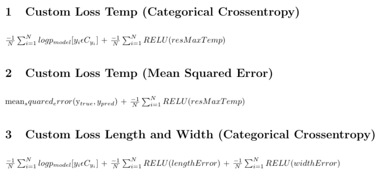
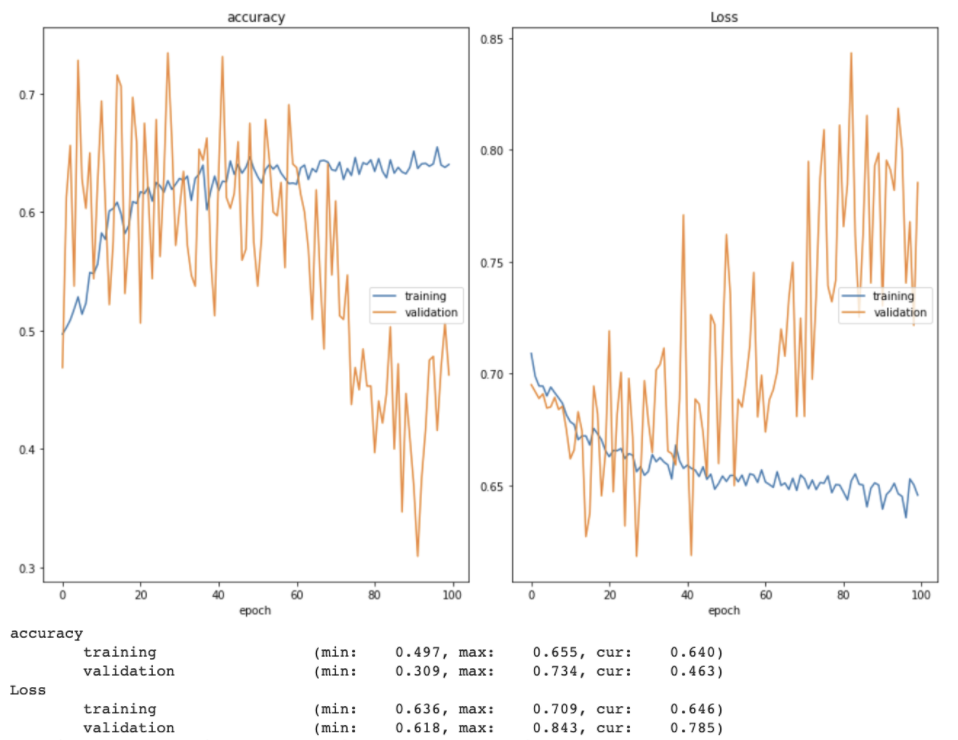
Above are the three loss functions I set out to test. The first, the foundation of which is the Keras categorical crossentropy loss function (first term), penalizes the model whenever the empirical maximum melt pool temperature is greater than the simulated maximum temperature. The second does the same, but uses the Keras mean squared error loss function (first term) as a foundation instead. When it came to actually coding a custom loss function with additional parameters in Keras (which typically only allows loss functions to take in the true and predicted labels), I used the associated code from “Physics-guided Neural Networks (PGNN): An Application in Lake Temperature Modeling” [1] as a guide, wrapping a function that used only the true and predicted labels as parameters in separate function that accepted the residual maximum temperature. The results of incorporating these functions into my model can be seen below.

The third loss function also uses the Keras categorical crossentropy loss function (first term) as a foundation. However, I was not able to test this one yet, as I am only able to measure the length and width of the experimental melt pools in pixels (as opposed to the unit used to measure the simulated melt pools, which I also could not find anywhere in the description of the data). I plan to discuss resolutions to this issue with Dr. Guo during our Monday meeting.

This week I also began writing my final technical report and preparing my final presentation.

Week 8 (7/12 - 7/18) Research Log

This week I defined several more physics-informed loss functions to test based on a variety of possible constraints:

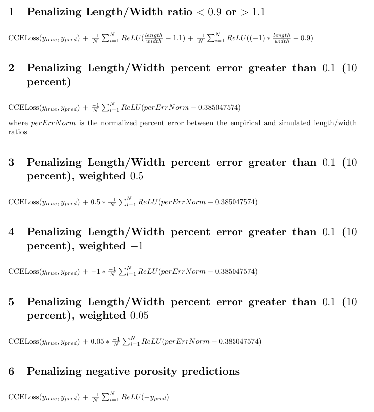
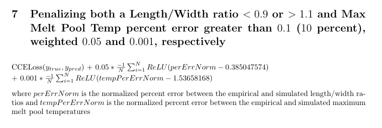
In the above functions, CCELoss(y_true, y_pred) denotes the regular training loss of a CNN that evaluates categorical cross entropy as a means of measuring the discrepancy between the predicted label for each image (y_pred) and the true label for each image (y_true). Since our model is sorting images into two classes, the loss due to categorical cross entropy is CCELoss(y_true, y_pred) = −t₁log(s₁) − (1 − t₁)log(1 − s₁), where t₁ and s₁ are the true label and predicted label for Class 1 and (1 − t₁) and (1 − s₁) are the true label and predicted label for Class 2. Unfortunately, the initial run of all of these versions of the model began to overfit to the training set after less than 10 epochs. I continued to experiment with giving greater weight to certain terms in the equation by adding coefficients, normalizing the physics-based data, and running each version of the model for more epochs at Dr. Guo’s recommendation.

I also continued to work on my final technical report for the REU program, as well as my final presentation.

Week 9 (7/19 - 7/23) Research Log

This week, I condensed the physics-informed loss functions I had experimented with thus far into the following five functions:

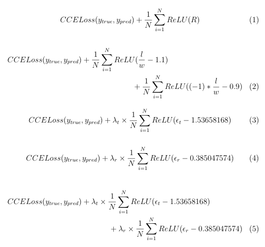
where CCELoss(y_true, y_pred) denotes the regular training loss of a CNN that evaluates categorical cross entropy as a means of measuring the discrepancy between the predicted label for each image (y_pred) and the true label for each image (y_true). The other variables are defined as follows:

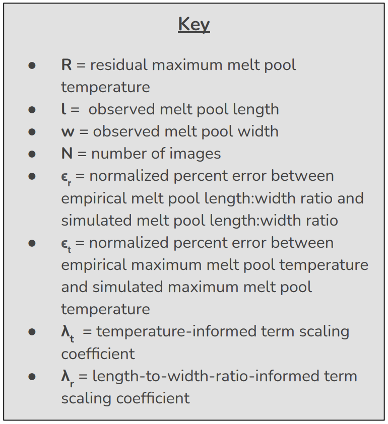
Equation (1) penalizes instances where the observed maximum melt pool temperature is greater than the simulated (ideal) maximum melt pool temperature. As the simulated length:width ratio was 1 for every melt pool, equation (2) penalizes any instance in which the observed length:width ratio of a given melt pool varies from 1 by more than 10 percent. Equation (3) penalizes any instance in which the normalized percent error between the empirical maximum melt pool temperature and the simulated maximum melt pool temperature exceeds 10 percent (prior to normalization). Similarly, equation (4) penalizes any instance in which the normalized percent error between the empirical melt pool length:width ratio and the simulated melt pool length:width ratio exceeds 10 percent (prior to normalization). Equation (5) is a combination of equations (3) and (4).

During the experimentation stage, some models had been set to train for longer than others. In order to ensure fair results, I decided that each version of the model should be set to train for 100 epochs with an early stopping point of 50 (based on validation loss). While most of the results I had gathered so far fit these specifciations, I allowed the versions that fell short of this to train for the necessary number of epochs. For each training session, the learning rate was set to 0.001 and the stochastic gradient descent method was selected as the optimizer. The results of these training sessions are shown in the tables below, wherein PICNN (physics-informed CNN) followed by a number denotes the version of the model that was trained using the physics-based loss function previously denoted by that same number (e.g. PICNN1 was trained using equation 1 as the loss function). The results for the baseline deep learning-only model (trained on the regular categorical cross entropy loss function) are also included for reference. The best weights (based on lowest validation loss) from each training session were used to generate predictions for the test set.

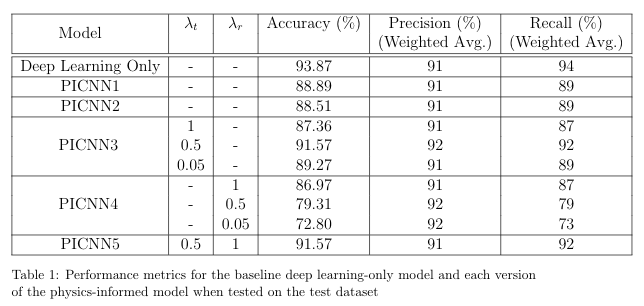
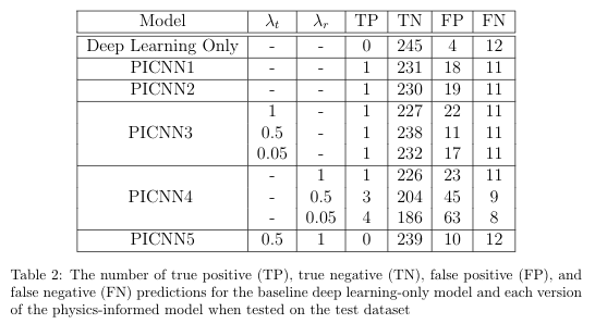
At this point the key findings are: (1) While this physics-informed model was not able to improve the predictive capabilities of the deep learning model in every respect, some versions were able to improve upon the precision of the baseline model (2) this improvement in precision was due to an increase in the number of true positive predictions and (3) this improvement in precision came at the expense of the overall accuracy of the model.

Moreover, this week Dr. Guo and I discussed the possibility of using my final technical report for the DIMACS REU program as the basis for an article that we can submit to an academic journal for publication, as well as a preliminary outline of what this paper would look like. After the end of the REU program, I intend to continue working with her and Vidita to further tune the physics-informed models and pursue the publication of our findings.

This Thursday, July 22nd, I gave my final presentation for the DIMACS REU program. The slides for this presentation can be found here. I also completed and submitted my final technical report to the REU program after receiving approval from Dr. Guo.

I would like to extend my sincerest gratitude to Dr. Guo, her graduate student Vidita Gawade, and the DIMACS REU Program for their support and guidance on this project. I would also like to thank the National Science Foundation; this work is supported by NSF grant CCF-1852215.