I'm Enver Aman. I am currently an undergraduate at Rutgers University majoring in math and CS (focusing more on math). This webpage is where I'll keep track of my progress on my project in DIMACS (Summer 2022) and other related stuff.
Outside of academic stuff, I play a lot of rhythm games! The only game I play daily is Arcaea (I'd like to say I've gotten pretty decent at it), but I also play Groove Coaster, CHUNTIHM, and WACCA, along with other stuff whenever I go to an arcade. I used to play Dynamix and Lanota too, but have stopped because I need to figure out how to transfer data between devices but have been too lazy to. I'm also an avid reader of manga/webtoons. I should probably catch up on some of the newer anime, but oh well.
I also really like listening to Touhou doujin music. I've been listening to a lot of rock stuff, so circles like Water Color Melody (actually, "常識的にかんがえて" has been stuck in my head all day!), Sally, Butaotome, TsuBaKi, and Touhou Jihen have been on my mind recently. Mili's "Key Ingredient" album has also been really nice and nostalgic. I'd actually like to start collecting some of these doujin albums, but shipping is pretty expensive right now. I'm always down for a good chat about Touhou/original doujin Japanese music!
My email: enver.aman@rutgers.edu
Here is some more DIMACS-related information:
I would like to thank Professor Alex Kontorovich for advising me and the DIMACS staff for supporting me in this research. Thank you also to the NSF: I am supported through grant NSF DMS-1802119.
I will be working on Markoff triples and the Strong Approximation conjecture. The idea of the project is to study solutions to the equation \[x^2 + y^2 + z^2 = 3xyz\] over \(\mathbb{F}_p\) (integers modulo \(p\)), where \(p\) is a prime number. The equation above is called the Markoff equation (yes! It's the same Markov). Solutions to the Markoff equation are called Markoff triples.
One can view the solution set of this equation as the variety (set of zeros) \(X^*(p) := \mathbb{X}(\mathbb{F}_p)\) of the polynomial \(x^2 + y^2 + z^2 - 3xyz\) over \(\mathbb{F}_p\).
On top of all this, there is a notion of "jumping" from one solution to others using what's called a Vieta jump. Starting from a Markoff triple \((x,y,z)\), we can jump to another Markoff triple by keeping two of the coordinates constant and solving for the third (there is usually a different solution because the equation obtained is quadratic in the third variable). For example, given the solution \((x,y,z)\), the following are all also solutions to the Markoff equation: \[(x, y, 3xy - z), \ (3yz - x, y, z), \ (x, 3xz - y, z).\]
We can then create a graph with \(X^*(p)\) as the set of vertices: connect two points \(a,b \in X^*(p)\) if one can Vieta jump from \(a\) to \(b\). The Strong Approximation Conjecture for Markoff triples states that this graph is always connected for each prime \(p\), except for the trivial solution \((0,0,0) \in X^*(p)\).
The question can be similarly formulated in \(\mathbb{Z}\). Markoff (or Markov, whichever you'd prefer) had shown in 1980 that, from the solution \((1,1,1)\), one can use these Vieta jumps to get to any other nonzero solution of the Markoff equation in \(\mathbb{Z}\), up to permutation of the coordinates and sign changes.
The Strong Approximation conjecture has been shown for most primes in a 2016 paper by Bourgain, Gamburd, and Sarnak (paper: https://arxiv.org/abs/1607.01530). The set \(E\) of primes that violate the conjecture above has been shown to be finite by William Chen in 2020 (paper: https://arxiv.org/abs/2011.12940). Our goal is to finish up the proof of the Strong Approximation conjecture by finding an explicit bound for \(E\) and computing the graph given above for primes less than this bound.
Week 1 (5/31/2022 -- 6/5/2022): I got to meet my roommates, my projectmates, and the other people at DIMACS. Unfortunately, I got sick this week so I haven't really been able to do much yet. I mostly rested up and got better this week. At the end of the week, I chose my project as described above.
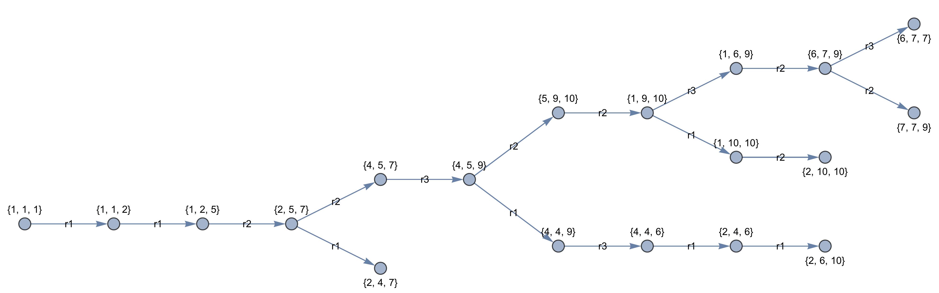
Week 2 (6/6/2022 -- 6/12/2022): I finished up a little (probably inefficient, but oh well :>) python script for creating the "Markoff trees" of \(X^*(p)\). The graphs have cycles in them since not all Vieta jumps can jump to vertices not already found. I call them "trees" because I didn't draw these jumps that brought you back to an earlier point.
Here's the Markoff tree for \(p=11\) below (that is, for \(X^*(11)\), the solution set of the Markoff equation mod \(11\)). As you'd probably be able to guess, these trees get pretty big for primes bigger than \(30\), so visualization beyond that point is probably hopeless.
I've also started to read the Bourgain, Gamburd, Sarnak paper (hereby called BGS16) I mentioned above. I'm trying to understand the details of the paper so I've been going along slowly. Hopefully I can get to the more meaty parts of the paper by the end of next week!
Week 3 (6/13/2022 -- 6/19/2022): The BGS16 paper has been a new challenge for me to understand! I feel like there are two main parts at play in the paper: the number theory part and the geometry part. I've mostly referenced another paper for the number theory part: the undergraduate thesis of Alexander López (2022).
We've introduced a "rotation" map \(\mathrm{rot}_1\) as the composition of a permuation map with a Vieta involution: \[\mathrm{rot}_1(x,y,z) = (x, 3xz - y, z).\]
We can view this as a linear transformation on the coordinates \((y,z)\) and notice that the matrix \[M(x) := \begin{bmatrix} 0 & 1 \\ -1 & 3x \end{bmatrix}\] pops out. Of interest are the eigenvalues (in \(\mathbb{F}_p\)) of this matrix: the characteristic polynomial of \(M(x)\) has determinant \((3x)^2 - 4\), which is really the only possibly trouble bit in \(\mathbb{F}_p\) (since square roots may not be defined).
This is where the motivation behind calling certain points \(x \in \mathbb{F}_p\) hyperbolic/parabolic/elliptic based on what the Legendre symbol \(\left(\frac{x^2 - 4}{p}\right)\) equals (\(1, 0, -1\), respectively). (Actually, Legendre symbols seem really cool! I'd like to learn more about them, but maybe later.) The point of these definitions is that the classification of \(3x\) corresponds to the number of eigenvalues that \(M(x)\) has.
From here, the paper discussed how many solutions to the Markoff equation there are with a fixed coordinate. In terms of the notation in my project description, this part discussed the size of the set \[C_j(x) = \{(x_1, x_2, x_3) \in X^*(p) : x_j = x\}.\]
The size of this set depends on the classification of \(x \in \mathbb{F}_p\). In summary, \(|C_j(x)| \approx p\) when \(x\) is either hyperbolic or elliptic, and \(|C_j(x)| \in \{0, 2p\}\) when \(x\) is parabolic, the choice depending on the residue of \(p\) modulo \(4\). These results actually give us an exact count for \(X^*(p)\): we have that \(|X^*(p)|\) is roughly \(p^2\).
The next part (geometry) was a lot scarier to me. I've been able to verify a lot of the statements with small choices of \(p\), but am struggling to understand the proof. Professor Kontorovich tells me not to worry about them, but I still feel a little uneasy with some of them. I have an idea that I'd like to pursue (that I've also told Prof. Kontorovich), but I'll reveal that next week! (cliffhanger :o (unless you're from the future :oo))
Week 4 (6/20/2022 -- 6/26/2022): Turns out my idea was incorrect 😓. The idea would have connected a computation on matrices over \(\mathbb{F}_p\) to elements of \(\mathbb{F}_p\), which would have turned the big question into something more general (and hence something that might have answers) and cut computation time in quarters!
Unfortunately, the theorems I was using weren't applicable: I failed to read the fine text about some of the conditions that weren't held. Oh well, I guess. There were some pretty neat results I got as a result of this guess, but I'm not sure if they will be relevant anymore.
On a side note, I've typed up my notes in LaTeX (and will continue to), which has helped organize my thoughts better than scribbles on scrap paper.
Was a little disappointed nonetheless, but I've been reminded that research is a challenge! Back to Python/Mathematica experimenting I go! I updated this a few days late, so here's a sneak peak of Week 5's Mathematica adventures ^_^.

Week 5 (6/27/2022 -- 7/3/2022): Do you remember the "Markoff trees" from the earlier entry? I've been looking at them (this time, completing cycles) trying to make some interesting observations. Actually, the picture above is (almost) the graph I talked about in the project description for \(p=19\) ("almost" because I ignored permutation maps). Call this the Markoff graph mod \(p\): denote it \(G_p\).
There have been some interesting things to see, particularly depending on the residue of \(p\) mod \(4\). I'm currently focusing in on the case where \(p \equiv 1 \pmod{4}\), since this case seems to be easier to deal with.
I've gotten something somewhat promising: I think I can show that there is a connected subgraph of \(G_p\) (called \(\mathcal{C}(p)\): the "cage") that is on the order of \(p^2\). This is pretty exciting because \(|X^*(p)|\) is also on the order of \(p^2\)! The bound is still kind of weak: here is some experimental data. (I'd be shocked if you could recover the bound from this graph 😄)

This is the stuff that I realized near the end of the week, after discussing some stuff with Prof. Kontorovich. I'd drawn lots of pictures in Mathematica earlier in the week to explore what was going on. Here are some of my favorites!


Week 6 (7/4/2022 -- 7/10/2022): I've been focusing on the rotation map \(\rot_1 = \rot\) that I mentioned a few weeks ago. Let \(\Gamma_1\) be the set generated by repeated compositions of \(\rot\). We can then treat \(\Gamma_1\) as a group acting on \(X^*(p)\): we're interested in the \(\Gamma_1\)-orbits of points \(a \in X^*(p)\).
We essentially have a graph \(H_p\) whose vertex set is \(X^*(p)\), and we connect \(a,b \in X^*(p)\) if there is a positive integer \(k\) such that \(\rot^k(a) = b\). (Here, \(\rot^k\) is shorthand for \(\rot\) composed with itself \(k\) times.) It's the case that \(H_p\) is a subgraph of \(G_p\). Visually, \(H_p\) looks like a bunch of disconnected cycles (see "Rotational Orbits for \(p=17\)" above!)
As a quick note, note that the cycle containing \((x,y,z) \in X^*(p)\) (alternatively, the orbit \(\Gamma_1 \cdot (x,y,z)\)) has the property that any other point in the cycle has first coordinate \(x\) as well. That is, \(\rot\) preserves the first coordinate of its input.
We can connect two cycles in \(H_p\) under a permutation map if there is a point in one cycle that is a permutation of a point in the other cycle. Our goal now turns into showing that \(H_p\) is connected in this way. (If \(H_p\) is a connected, then so is \(G_p\)!) (Also, this has been a lot of setup so far... but it's worth it I swear)
This week, I observed \(H_p\) alongside some experimental data, and I think I almost fully understand the structure of \(H_p\). Understanding the structure of \(H_p\) is important (BGS16 concerns itself with \(H_p\)). I've been able to...
Call this lower bound \(L(p)\). Currently, this lower bound \(L(p)\) implies that \(\mathcal{C}(p)\) contains just about half of the elements in \(X^*(p)\). Here is a graph of \(L(p) / |X^*(p)|\) over the first \(10000\) primes (it's the small blue dots).

We eventually want this ratio to be more than \(1\), but as it stands, the ratio seems to vary in a "strip"; (at least for larger \(p\)) between about \(0.47\) and about \(0.65\).
To be honest, I'm not really sure where to go from here: after discussing with Prof. Kontorovich, I've decided to return to looking at the BGS16 paper (which has become a lot more comprehensible after all this motivation!) and to try to upper bound \(|X^*(p) \setminus \mathcal{C}(p)|\). Remember, if we can show that this quantity is less than \(p\) (William Chen), then we're done!
I had a relaxing weekend and am ready to dive back into algebraic geometry land!
Week 7 (7/11/2022 -- 7/17/2022): I have returned to the BGS16 paper, focusing on explicitly finding mentioned constants in the paper. This required use of a certain result from algebraic geometry: the "Riemann Hypothesis over Finite Fields", otherwise known as the Hasse-Weil bound.
The bound states that, for a curve \(C\) of genus \(g\) with "certain conditions" (in quotes because I don't fully understand what these conditions are haha), the number of points \(N\) of \(C\) over the finite field \(\mathbb{F}_q\) is bounded by \[|N - (q+1)| \leq 2g\sqrt{q}.\]
Using this bound, Bourgain, Gamburd, and Sarnak show that, for any \(\delta > 0\) and for most primes \(p\) (primes in a set \(P_\delta\) depending on \(\delta\)), points of the form \((x,y,z) \in X^*(p)\) are connected to the cage if \(\ord(\rot(x)) \geq p^{1/2 + \delta}\).
The issue is that the set \(P_\delta\) seems hard to describe. Following along the arguments given in BGS16, refining parts where big-\(O\) estimates were used, I've been able to show the following:
Choose integer \(N > 0\) and real \(\delta > 0\) (pref. smaller than \(1/2\)). For each prime \(p < N\), the point \((x,y,z) \in X^*(p)\) is connected to the cage if \[\ord(\rot(x)) \geq C(\delta, N) \cdot A p^{1/2 + \delta},\] where \(A\) is some constant estimating the genus of a specific curve.
The constant \(C(\delta, N)\) (constant in \(p\), that is) can be written as a product of two functions \(C(\delta, N) = 2\alpha(\delta) \beta(N)\). The function \(\alpha(\delta)\) actually doesn't increase too much as \(\delta\) decreases: The function \(\alpha(1/n)\) seems to grow a little faster than \(\log n\) (but not quite any power of \(n\)).
On the other hand, \(\beta(N)\) seems to grow much faster? I'd have to check more specifics, but every value of \(C(\delta, N)\) I've computed so far has had most of its contribution from \(\beta(N)\).
You'll notice that I've skipped talking about \(A\). I (currently) have no idea how to calculate \(A\) explicitly. The hope is that \(A\) is small, like \(2\) or \(4\). The bound above would be irrelevant if \(A\) were too big.
The condition on \(\ord(\rot(x))\) above is only really useful when \(C(\delta, N) \cdot A < \sqrt{p}\), so in fact we obtain that points of \(X^*(p)\) with a large enough order can be connected to the cage, under the condition that \(p\) lies in some finite interval of the form \((N', N)\).
There is only two weeks left in the REU, but I feel like there's still so much to do...