
| Name: | Anna Cusenza |
|---|---|
| Email: | ascusenza@g.ucla.edu |
| Home: | University of California, Los Angeles |
| Project: | Data Driven Dynamics |
| Mentors: | Konstantin Mischaikow , Marcio Gameiro - Fuzeto, William Cuello , Ewerton R. Vieira |
About My Project
For this project I will investigate ways that can potentially be more efficient when computing dynamics from a set of data. The data of interest is from a multi-parameter, nonlinear dynamical system. Such systems have quite complicated behavior. One method which is used to analyze data is to discretize the information via a decomposition of the compact phase and parameter space into square grids. This makes the information being studied finite and computable.
With this decomposition, a directed graph which corresponds to the map is created, where each node is one of the square grids in the phase space, and the directed edges denote where each grid maps to under the dynamical system, depending on the input from the parameter space. Below are images (source)to explain this concept.
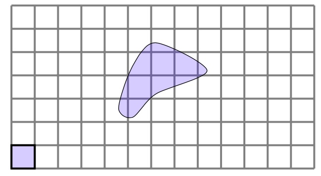
Here we have a decomposition of some space into square grids. The spaces we will analyze for the purposes of this project will always be compact (closed and bounded). The purple square in the bottom left is the grid to which we apply a map. The purple blob in the middle is the image of the square under the map.
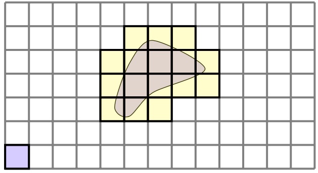
We now cover the image with the cubical sets that intersect the image. This is called and outer cover of the image. We see that the cubical cell in the bottom left maps to these cells which form an outer cover of its image. So we add directed edges accordingly to denote this.
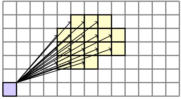
To simplify this directed graph, and get a more coherent picture of the global dynamics, we collapse all the strongly connected path components to one node. This then gives us the Morse graph, and makes it clear what are the non-recurrent dynamics. Conley index theory, which utilizes algebraic topology, is also used to understand properties of the dynamical system, such as the recurrent dynamics. For a description, see this file
Research Journal
Week 1: May 24 - May 28
This week I have been working on familiarizing myself with the language and terms that come up often in work related to this project. As of now I am also working on installing the software needed (Jupyter Notebook), and trying to figure out why some programs are not downloading on my computer (ugh!). I am also reading this paper for an intuitive understanding of what I will be doing over the next few weeks.
Week 2: May 31 - June 4
We managed to resolve all my technical difficulties! I spent time with my mentors going over the code developed for previous research, to get familiar with the methods used. You can find the code I'm looking at here. Throughout my project I will be using and modifying the programs available via the link. I also started reading this paper. You may need to log in to a campus VPN to access the paper.
Week 3: June 7 - June 11
Finals week at UCLA.
Week 4: June 14 - June 18
I am reading the papers previously listed more thoroughly, and going over relevant topics that I don't have experience with. Papers on this topic of dynamics have employed tools from algebraic topology, and include a discussion on homology. I am not very familiar with homology so I am also spending some time learning about that. Wikipedia is a good place to start for the intuition, then I plan to read from this and I may go into Hatcher. I am also spending more time understanding the code listed above.
Week 5: June 21 - June 25
This week I did some more studying regarding homology. It is really helpful to know some topology and group theory. I also started working on implementing a graph where the discretization of the phase space is via a Voronoi decomposition. In the description of my project I mention how previous work decomposed the phase space into a square grid, and how a directed graph was created to approximate the behavior of a system so that the dynamics created by the system can be studied with computational methods. The goal for this project is to investigate whether using a Voronoi decomposition of the phase space will give a more efficient way to analyze dynamics, especially in higher dimensional systems. As I work on the programming I am currently working with the Leslie map, and we hope to apply the methods developed in this project to data collected from real studies in robotics and biology, for example.
Week 6: June 28 - July 2
I started reading more in depth this book on computational homology, starting with chapter 2. I figured out how to visualize Voronoi cells, with a great help from this nice tutorial on daniweb.com.
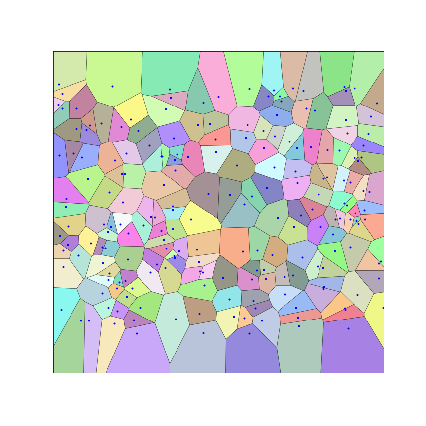
With this Voronoi decomposition, I can now make a directed graph as described before, where each node is now representing a Voronoi cell rather than a square cell. For the last few days of this week I have been working on making my new code less expensive and time consuming. Here I have accepted what it means to have code that works but at the same time sucks, something I declined to acknowledge when taking programming classes. To make my code run faster, I have so far used dictionaries which helped immensely. With even larger sample sizes, which I have not used so far, we may need some more intricate computational tools which I will describe as I approach them in the upcoming weeks. At this point, my code with the Voronoi cells is slower than the code which utilizes square grid decompositions.
Week 7: July 5 - July 9
With the Voronoi decomposition I can now plot the morse sets in the phase space. Here is an example of a morse graph for the Leslie map with the corresponding morse sets (colored the same as the morse graph).
Morse graph:

Morse sets:
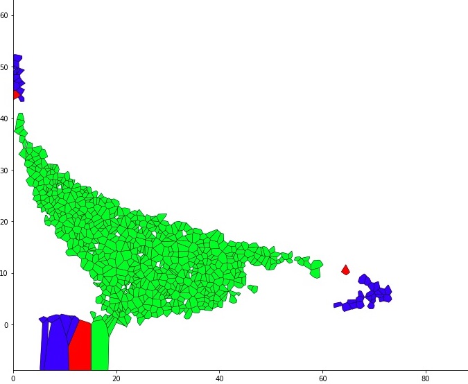
Where in this example 5500 Voronoi cells decompose the space $[0,90]\times[0,70]$ and the size of the set $X$ for which we apply the Leslie map is 40500.
Notice how the plotted morse sets above have some gaps. For example, the green region should not have those white holes. Our reference is the plot of the morse sets using the cubical decomposition of the phase space:

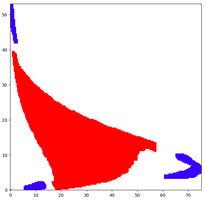
Where the phase space is the same $X = [0,90]\times[0,70]$, and the number of subdivisions of the phase space is 16, which means there are $2^{16}$ cubical cells.
The reason I am getting these gaps may be because $X$ is too small in proportion to the number of Voronoi cells, so that I don't have a value $x\in X$ which will map to one of the white holes, even though there is some value in $[0,90]\times[0,70]$ which maps to them. To hopefully fill in these gaps I will utilize the method of nearest neighbors. This means I will modify the map graph to also include edges that point to the image of nearest neighbors, and to the nearest neighbors of the image of the nearest neighbors, and see how this compares to what I had before. I have discussed with my mentors the potential of using the method with Voronoi cells to interpret data that is collected in research in ecology and robotics. To improve on the computational cost of my program I am also going to use multiprocessing. I have not gotten this to work yet..!Week 8: July 12 - July 16
Making use of the multiprocessing is proving difficult, for some reason it is not working on my computer. I am testing which ratio of number of cells to sample sizes yield optimal results. I am also testing my program with other maps, that are less chaotic than the Leslie map.
I also am working on some mistakes that my mentors and I have noticed with my nearest neighbors implementation. It looks like so far that when using the method of nearest neighbors, the morse sets are larger, and there are fewer of them. I will need to investigate how many nearest neighbors gives the most accurate result, and what is the optimal ratio of the number of Voronoi cells to the size of $X$ with this method. Since I am having trouble making my programming faster, it may be hard to experiment with many large sets!Week 9: July 19 - July 23
We had final presentations this week, marking the official end of the DIMACS program.
Post Program: July 24 - September 1
I continued with my project for a few weeks after the official end of the program. Below is an outline of my main points of progress.
I have found a 'bug' in my program, where I have been computing more dictionaries than I needed to. This helped with the time cost a lot!
I have tested the methods developed over the course of the program on different maps besides the Leslie map, like the Logistic map, and on weather data collected from various locations such as Tuscon, AZ, Seattle, WA, and multiple counties in California. Testing my code with data besides the Leslie map helped me find more bugs in my code!
When generating Voronoi cells using randomly sampled points in the phase space, the Voronoi cells are often quite irregular. To get cells that are more uniform, you start first with any sample of generating points for the Voronoi cells. Then, you iterate the following process until they are as regular as need be: (For $m$ dimensions) For each polygonal cell $P$, consider its vertices $\{v_1,\dots,v_n\}$. For each $i\in \{1,\dots, n\}$, take the average $c_i = \overline{\{v_{i,j}\}_{j = 1}^{m}}$ to get the point $c = (c_1,\dots,c_m)$. This will be the new generating point of the polygonal cell P. So far, this process has only been implemented in 2 dimensions.
I also generalized the code which plots the Morse sets and Morse graphs to work in $n$ dimensions generally, and used it to compute the Morse Sets for the Leslie map in 3 dimensions. For this, I made use of the Python library pyvoro, which is the python version to Voro++.
That wraps up my research this summer! As you may have noticed, there are still questions to be answered, and work to be completed. I am excited to hear about any progress on this project going forward, if the previous work proves interesting enough to continue! :-)
References & Links
Funding
This work was carried out while the author was a participant in the 2021 DIMACS REU program at Rutgers University, supported by NSF HDR TRIPODS award CCF-1934924.